 ETS New Mexico Course, 2023It’s been said that every map contains a story and every good story includes a map. Whether you use Apple Maps, Google Maps, MapQuest, or a good old-fashioned paper map, we can all agree that we’d be lost without them. But maps can do much more than just help you get from point A to point B. Maps can be powerful interpretive programming tools, and NASA makes some incredible maps!
At Earth to Sky, we use maps to connect the wonder of science with the power of place. Recently, our intern Brigitte created this brand-new guide to making natural-color maps from NASA’s Landsat Mission images. Follow the steps below to create your own map or watch the tutorial from our Science in Your Pocket webinar on May 16th, 2025 “A View from Space: Making Your Own Landsat Map”!
Download existing maps on the Earth to Sky Landsat story page.
Software
For this tutorial, you will need two free open-source softwares: Quantum Geographic Information System (QGIS) and GNU Image Manipulation Program (GIMP).
If you or your organization have a license to Photoshop, you can try the Photoshop version of the tutorial.
Workflow
Follow the 5 steps below to create a map of your own. This process will take around 2 hours the first time.
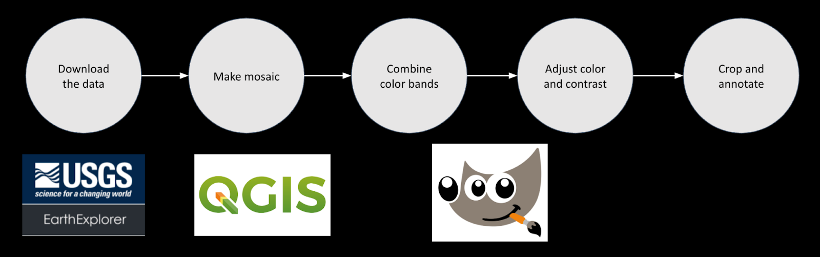
Step 1: Downloading the Data
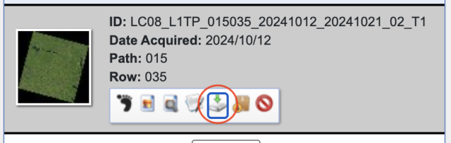
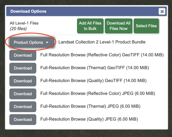
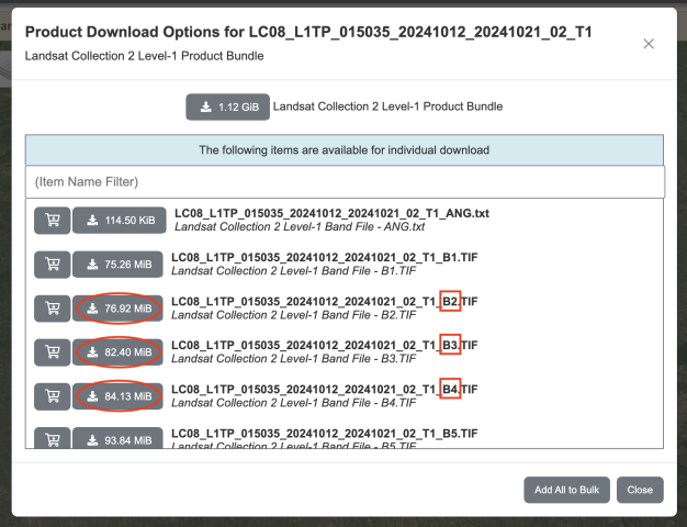
This tutorial will retrieve Landsat data from USGS Earth Explorer. First, you will need to make a free profile and set up your account. After making sure you are logged in, follow “Part 1: Downloading the Data” from NASA Landsat’s Creating a Landsat Image tutorial. In Step 7, after clicking “Product Options,” you can select which individual files rather than the entire package. For natural-color, we want bandcombo B2 (blue) B3, (green), and B4 (red). The files are all GeoTiffs (Tagged Image File Format), which means they include georeferencing data.
Step 2: Mosaicking – QGIS
- Open QGIS
- “New Project” (icon at upper left)
- The goal of this step is to make three mosaics, one for each color. You will do the following steps three times (once for B2, once for B3, once for B4).
-
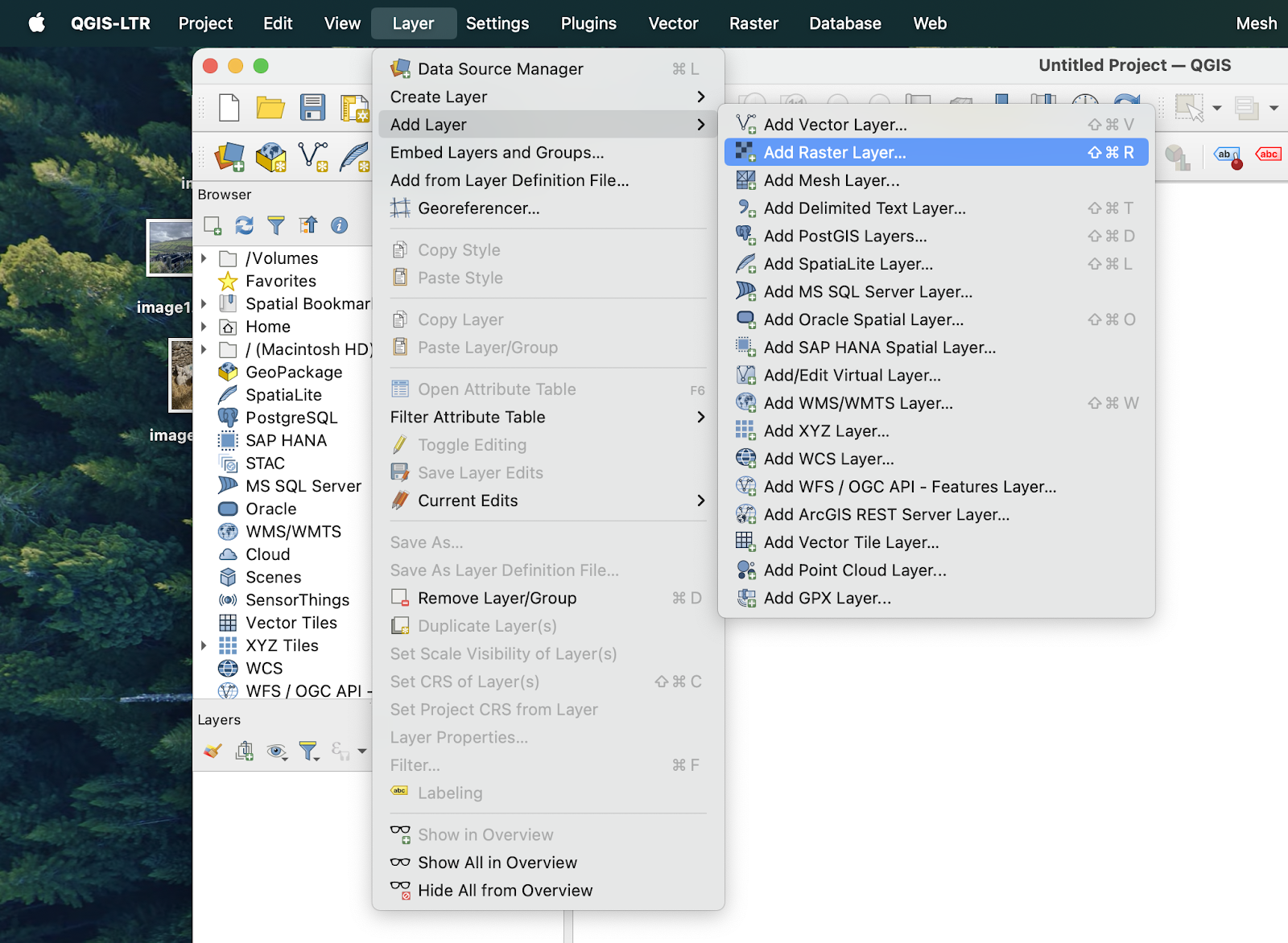
- “Layer” → “Add Layer” → “Add Raster Layer…” → Next to “Raster dataset(s)”, click the “Browser” icon. → select all images (of one bandcombo, i.e. select all B2 tiff) → Click “Add” then once they pop up in the background you may click “Close”
-
- You can reorder the layers front to back by dragging them up or down in the lower left “Layer” panel. If one image has clouds or the seam is very visible, etc. you may be able to cover it up with another image
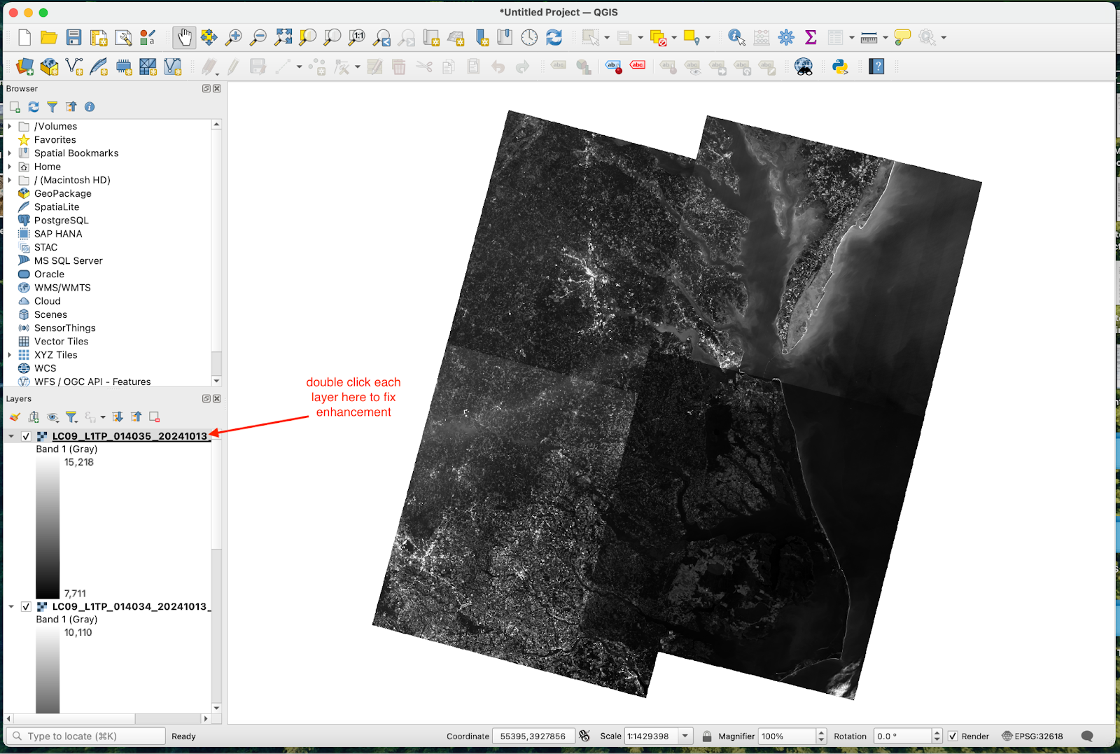
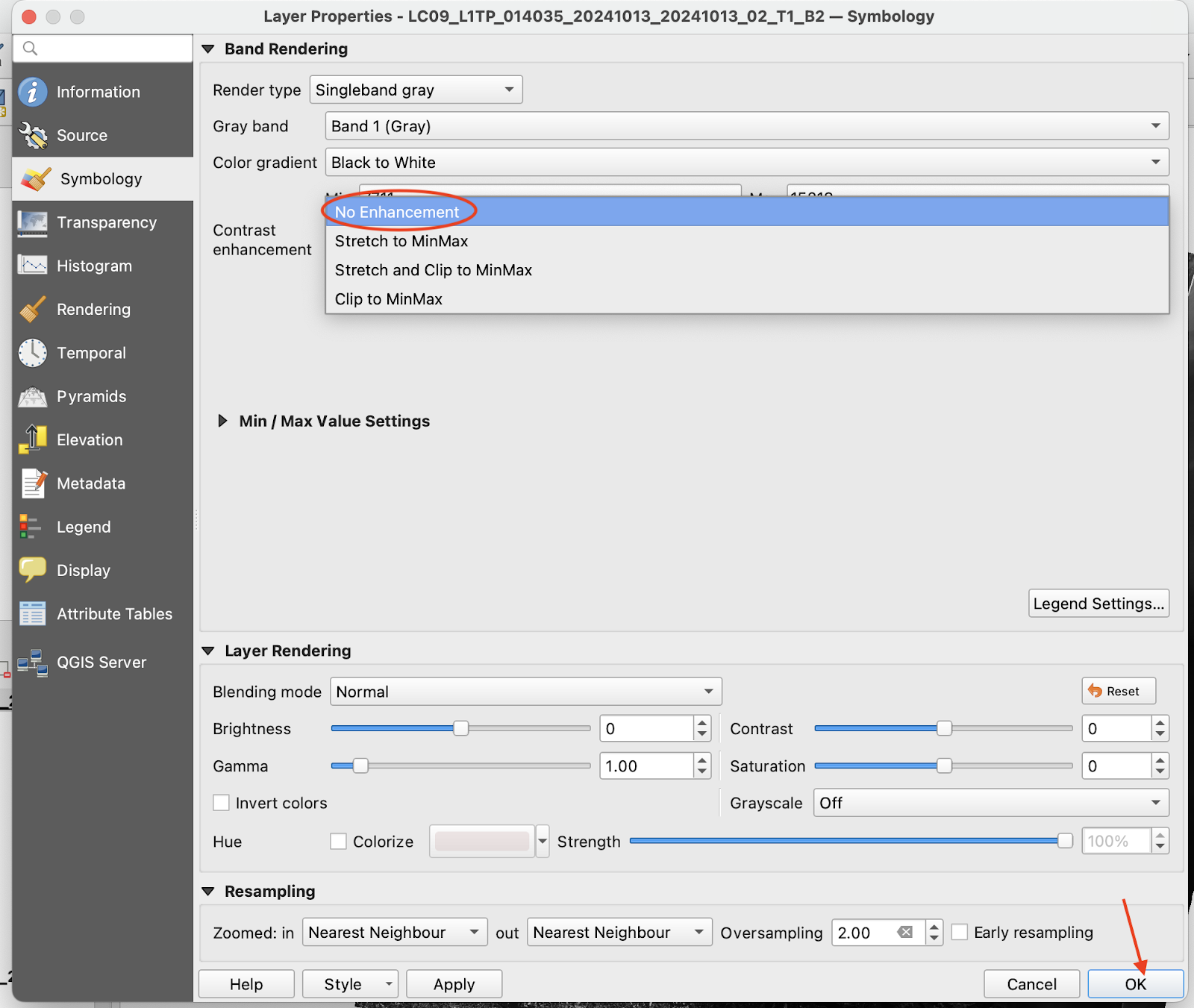
- Double click each file name (in the lower left “Layer” panel) and set “Contrast Enhancement” to “No Enhancement” then click “OK.”
-
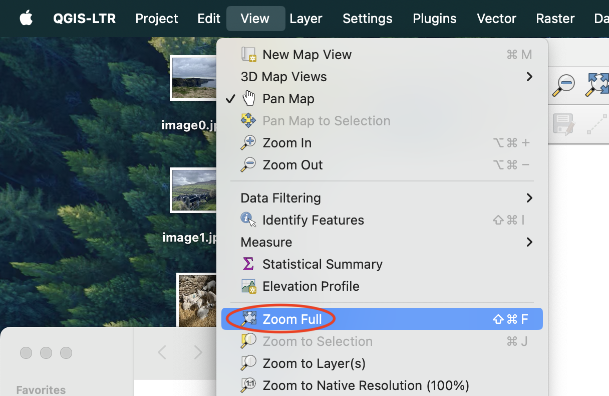
- To get the entire image centered, click “View” → “Zoom Full”. This will ensure all the images are aligned when we open them later on.
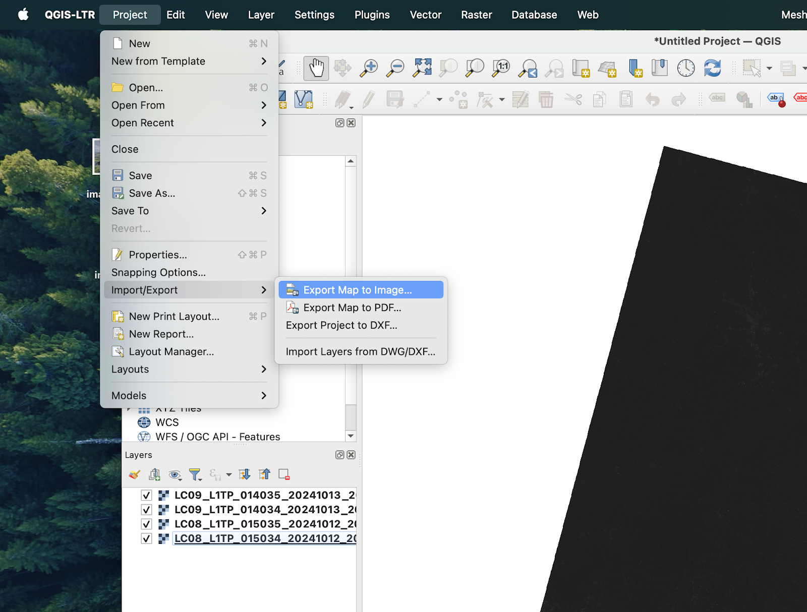
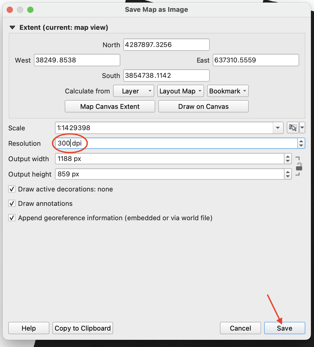
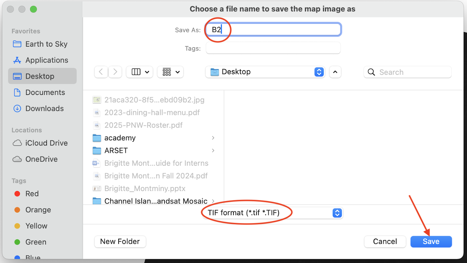
- “Project” → “Import/Export” → “Export Map to Image” → set “Resolution” to 500 dpi → “Save” → name the file (ex. B2), select the location, and select .tif
- The resolution depends on your map area, computer storage capacity, and desired outcome. Feel free to mess around with the resolution a bit.
Now, you should have three mosaics saved as .tif files, one for each bandcombo (B4, B3, B2).
NOTE: QGIS may save xml files into your folder for each individual file. You can ignore these.
Step 3: Merging Channels – GIMP
The goal of this step is to combine the three mosaics you just made into one mosaic that is RGB.
- Open GIMP
- “File” → “Open” → select your B2, B3, and B4 mosaics → “Open” → wait for all three images to load, this may take a moment and there may be other windows to pop up, but they should automatically close)
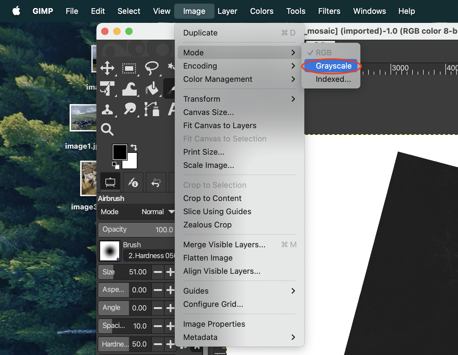
- At the top area, you should see three tabs (one for each of your mosaics). One by one, go to each image (by clicking on it in the tabs) and click “Image” → “Mode” → “Grayscale”. Make sure you do this for all three.
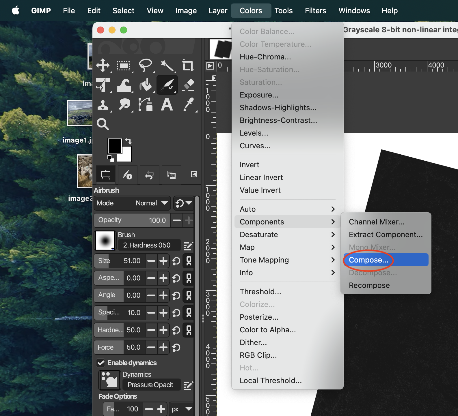
- Now combine the three mosaics into one full-color mosaic.“Colors” → “Components” → “Compose” and wait for a smaller window to pop up.
- Assign each bandcombo mosaic to the color using the dropdown buttons (red is B4, green is B3, blue is B2) → “OK”
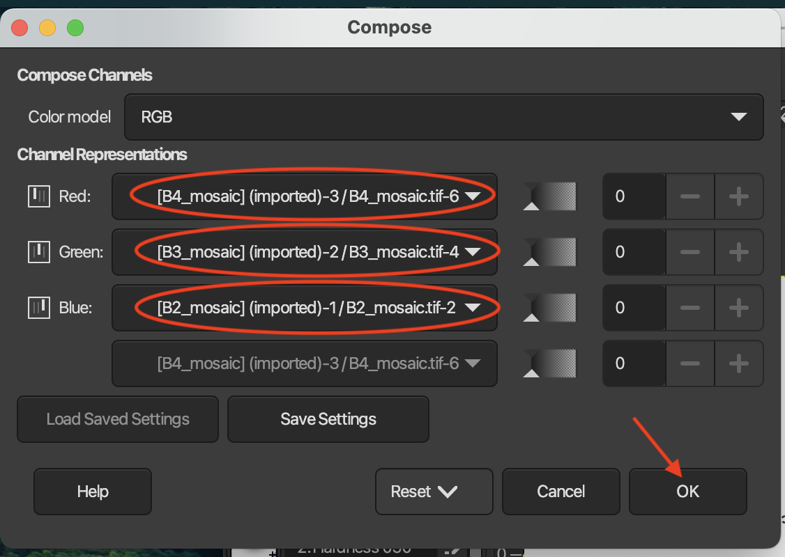
Wait for a new file to open (it will still look all black, should not be bright colors yet)
Step 4: Adjusting Color – GIMP
The goal of this step is to adjust the contrast and colors to create our full natural-color map.
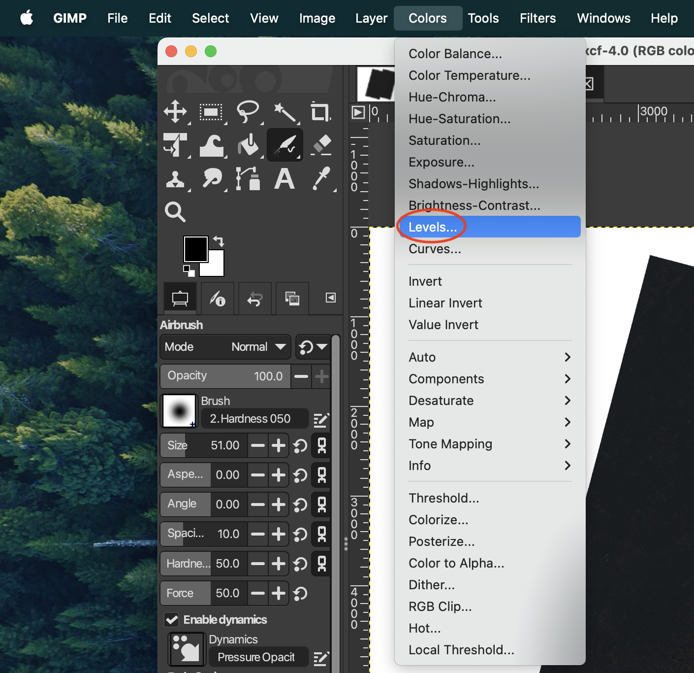
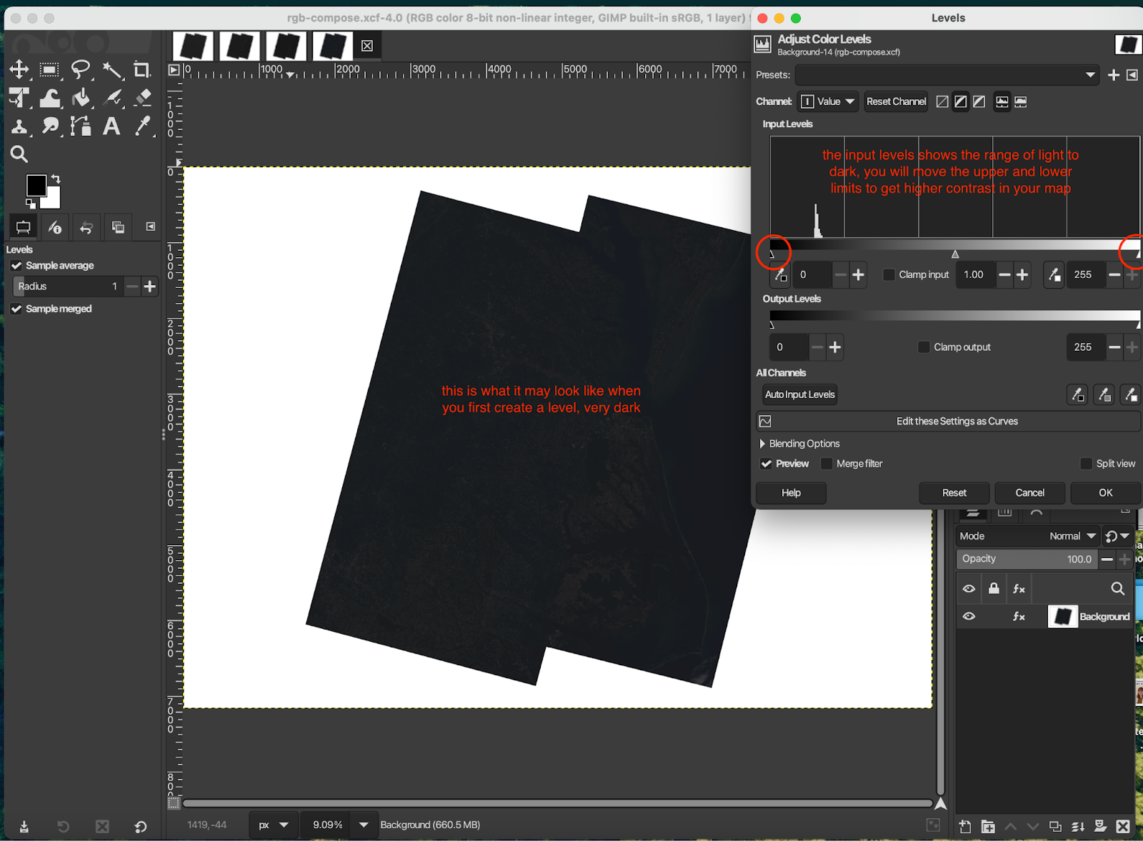
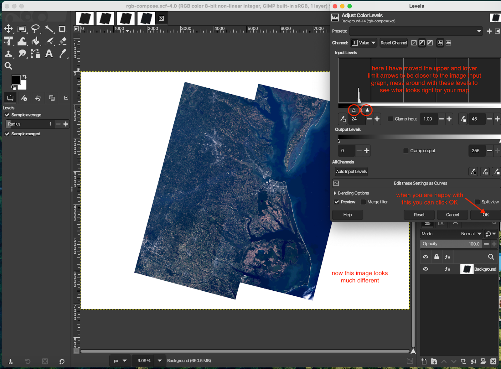
- “Colors” → “Levels…” → The window that pops up will have a graph for the input levels, we want to manually adjust the input level high and lows (light and dark) by moving the arrows right below the “Input Levels” graph (see images below). The goal is to lie on either end of the spikes on the histogram. Mess around with these levels until the contrast on your map allows you to see more details → “OK”
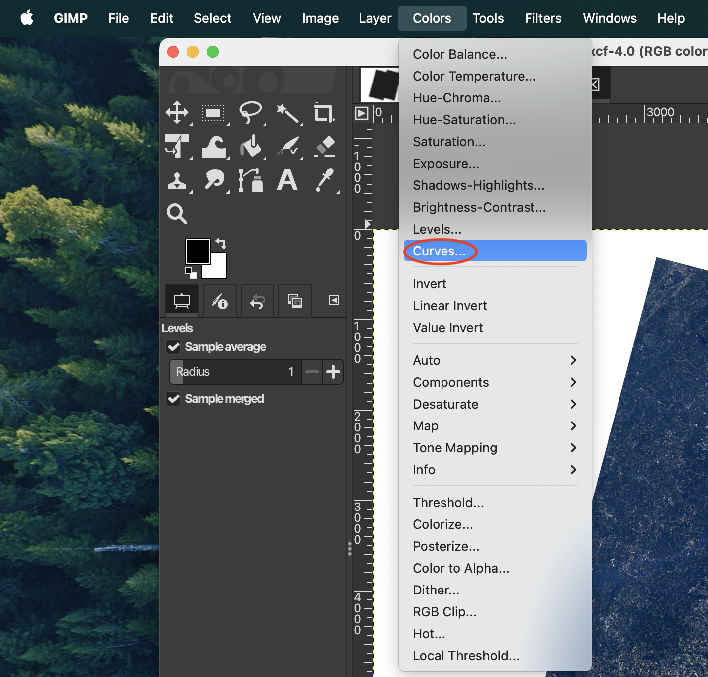
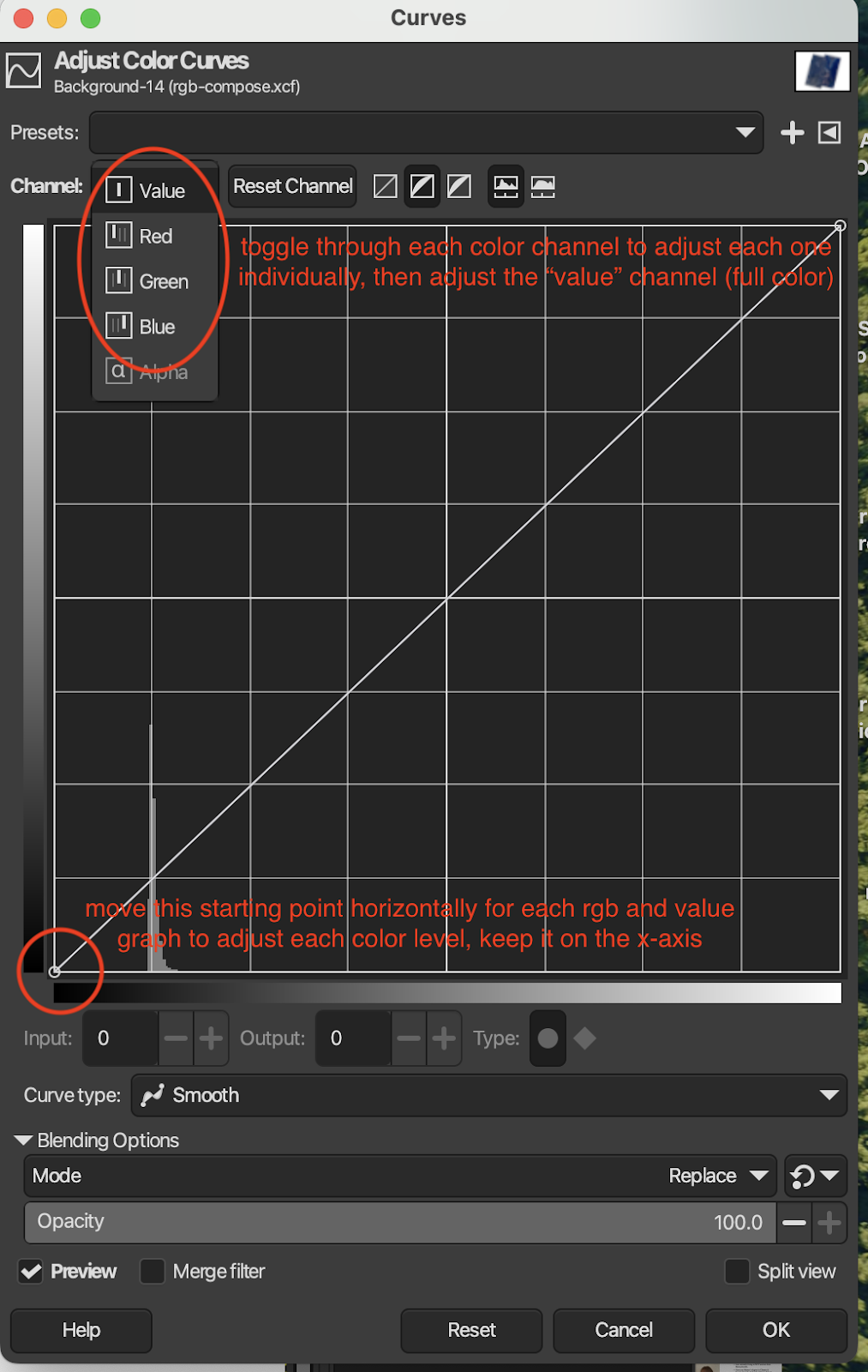
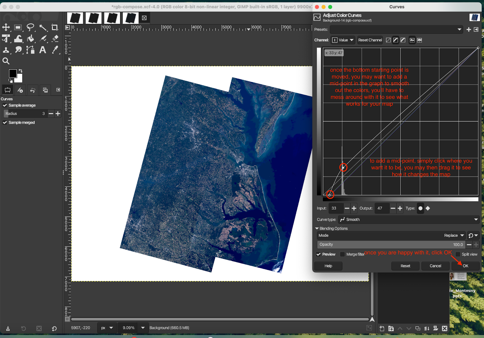
- “Colors” → “Curves…” → A small window will pop up that will allow you to manually adjust rgb curves and the total curve. Adjust the first point of each curve to sit between the start of the graph and the first major histogram spike. You can toggle between each color (red, green, blue, total) with the dropdown menu next to “Channel”. On the “Value” channel, add a point to the histogram to smoothen out the colors by clicking on the histogram. You can move this point up and down to adjust the brightness. Again, mess around with these graphs until you are happy with how your map looks.
- File → Save → this will save your work as a xcf file format
- File → Export → you may choose to save it as a png, jpg, etc.
Step 5: Crop & Add Annotations
Time to finalize your map!
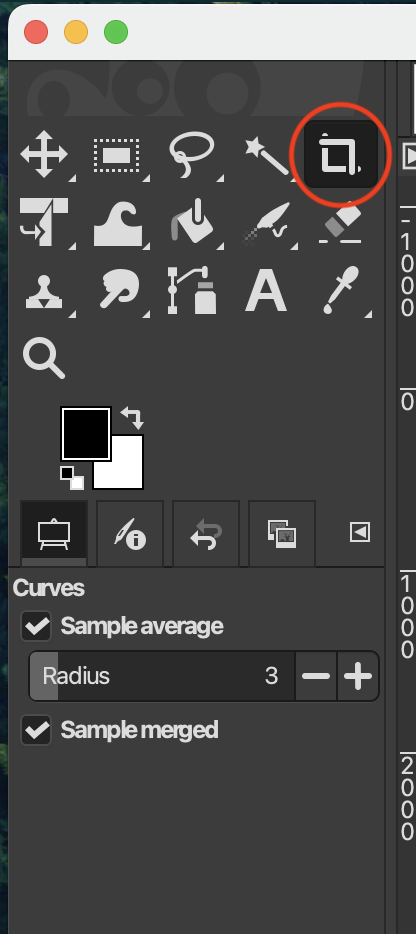
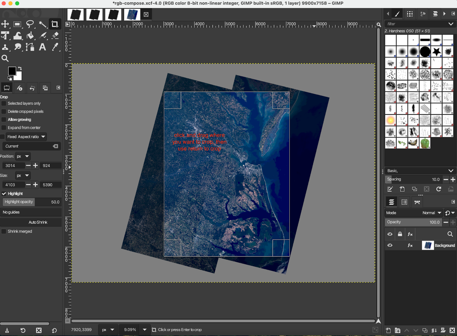
Cropping: select the crop icon in the upper left hand toolkit, then click and drag on your map where you want to crop
Annotations you may want to include:
- Name of your region
- Observing satellite (Landsat 8/9)
- Data acquisition date
- North arrow
- Scale bar
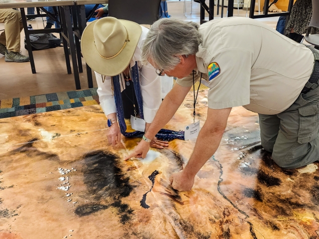
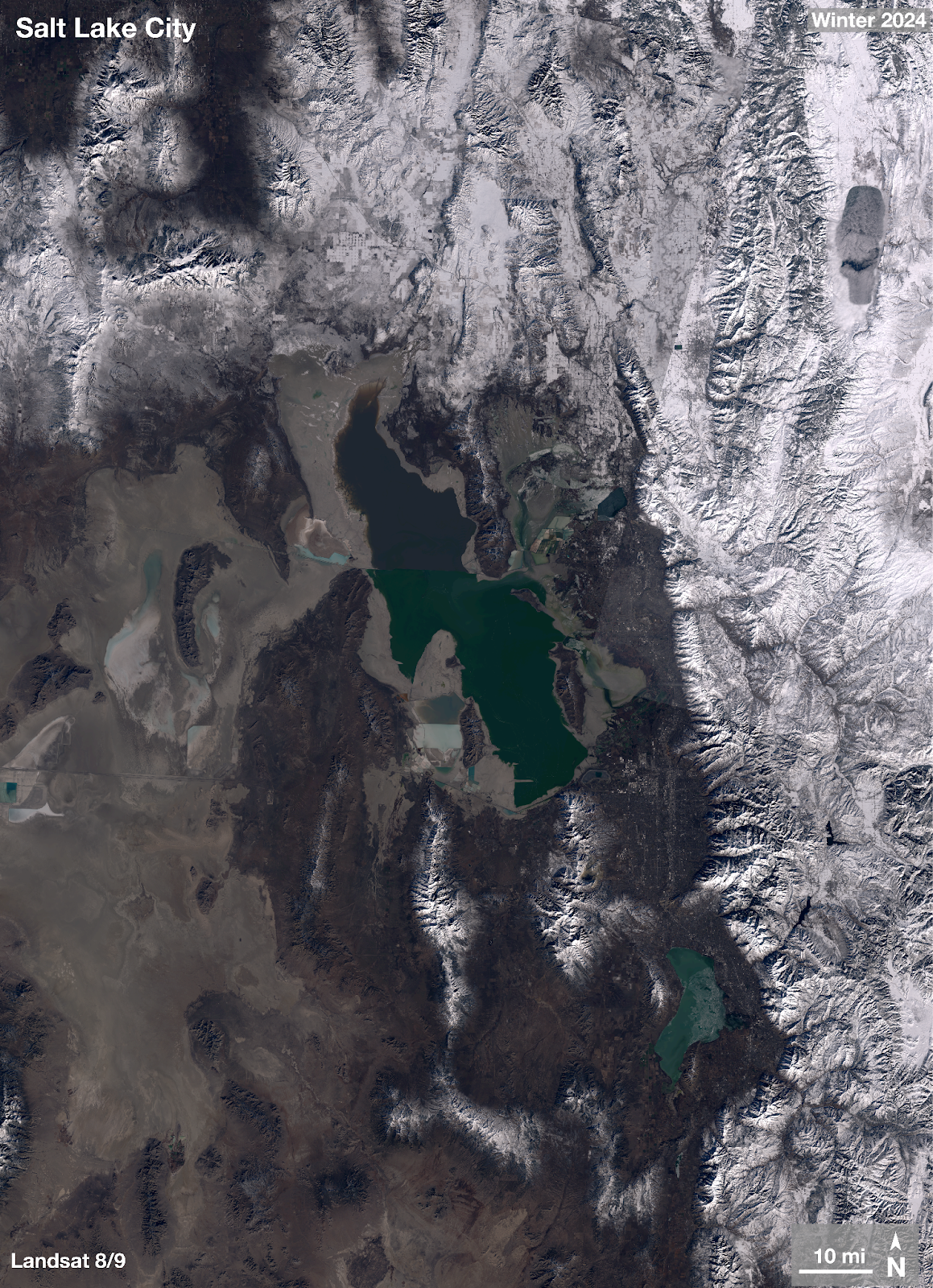
Here's an example!
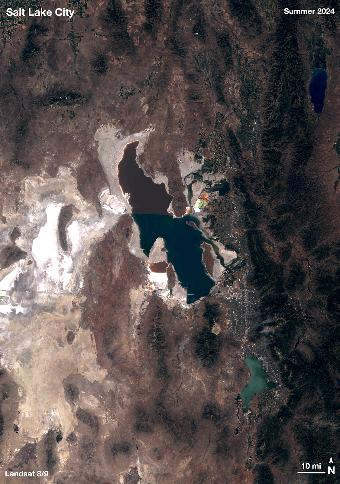
Made by Brigitte Montminy

Brigitte Montminy was a Climate Interpretation Intern working with Earth to Sky from August 2024 to May 2025. With a Bachelor’s degree in Astrophysics and a Master’s degree in Climate & Society from the Columbia Climate School, she is a science nerd with a specific love for maps. From mapping Jupiter’s polar clouds to Earth’s beauties, Brigitte is a fan of all types of maps. She is also currently working as a Climate Media Specialist at The YEARS Project, putting out a weekly newsletter and action toolkit.
Resources:
-
Earth to Sky Images | Landsat Science → collection of Landsat mosaics made for ETS
-
Creating a Landsat Image Using Photoshop w/ Mike Taylor | ETS Webinar (must be signed in)
-
Storytelling with Satellites - Landsat - Hawaiʻi Island w/ Ginger Butcher | ETS Webinar (must be signed in)
-
Creating a Landsat Image | NASA Landsat Science → great tutorial showing how to make a natural- or false-color Landsat image (note: not for mosaics)
-
Landsat Case Studies 2018 | NASA Landsat Science → learn about some of these tangible benefits of Landsat
-
Band Combination Interactive | NASA Landsat Science → online tool to visualize different Landsat band combinations using five different bands: blue, green, red, near-infrared, and short-wave infrared
-
What are the band designations for the Landsat satellites? | U.S. Geological Survey
-
What is the naming convention for Landsat Collections Level-1 scenes? | U.S. Geological Survey
- Landsat 8 Swath Animation | U.S. Geological Survey